Closer look into Learning Algorithm of a Neuron
[latexpage]
In perceptron model weights are changed to get a better set of weights. In multi-layer neural network this algorithm won't work and we don't use perceptron learning algorithm.
For multi-layer nets the objective is the actual outputs values reaching target output values.
Linear Neurons
The neuron has a real-valued output which is weighted sum of its inputs:
\begin{equation} y = \sum_{i}{x_i w_i} = W^T X \end{equation}
$W$ - Weight vector
$X$ - input vector
The aim will be to minimize the error. Error in this case is the squared difference between the desired output and the actual output.
Delta Rule & Iterative Algorithm
\begin{equation} \Delta w_i = \varepsilon x_i (t - y) \end{equation}
where:
$\varepsilon$ - learning rate
$t - y$ - (difference between the target and the estimate, i.e. the residual error)
Based on iterative algorithm delta rule adjustments will be done in the system to ensure that weights are adjusted by $ \Delta w_i $ with each iteration which should lead with to better result in case of Linear Neuron.
Note: (Deriving Delta Rule is explained separately)
Error Surface of a Linear Neuron
Assume the space where "all the horizontal dimensions" correspond to the weights and a vertical dimension corresponds to the error.
In this case errors made on each set of weights would define the error surface, which is a quadratic bowl.
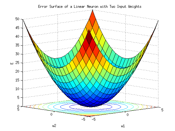
You can get the same on octave, using the source code:
vx = [-5:0.5:5];
vy = vx;
[x, y] = meshgrid(vx, vy);
z = x.^2 + y.^2;
surfc(x, y, z)
xlabel('w1')
ylabel('w2')
zlabel('E')
title('Error Surface of a Linear Neuron with Two Input Weights')
Logistic Neurons
\begin{equation} z = b + \sum_{i}{x_i w_i} \end{equation}
\begin{equation} y = \dfrac{1}{1+e^{-z}} \end{equation}
Deducing the delta rule
In order to find the derivatives needed for learning the weights of a logistic unit we need to find the quation for the following:
\begin{equation} \Delta w_i = \dfrac{\partial E}{\partial w_i} \end{equation}
using the chain rule, we would get:
\begin{equation} \dfrac{\partial E}{\partial w_i} = \sum_{n}{\dfrac{\partial y^n}{\partial w_i} \dfrac{\partial E}{\partial y^n}} \end{equation}
Another usage of chain rule and we would get:
\begin{equation} \dfrac{\partial y}{\partial w_i} = \dfrac{\partial z}{\partial w_i} \dfrac{d y}{d z} \end{equation}
By definition of $y$ and $z$ we would obtain that:
\begin{equation} \dfrac{\partial z}{\partial w_i} = x_i \end{equation}
\begin{equation} \dfrac{d y}{d z} = y (1 - y) \end{equation}
which means that:
\begin{equation} \dfrac{\partial y}{\partial w_i} = \dfrac{\partial z}{\partial w_i} \dfrac{d y}{d z} = x_i y (1 - y) \end{equation}
wrapping this up to the main question:
\begin{equation} \Delta w_i = \dfrac{\partial E}{\partial w_i} = - \sum_{n}{x_i ^n y^n (1 - y^n)(t^n - y^n) } \end{equation}
By original delta rule, applied on linear neuron we can interpret this result as a delta rule, adjusted by $y^n (1 - y^n)$ - the slope of the logistic function.
Learning by Randomly perturbing weights
One way to adjust the weights would be to do a random change on one of the weight and investigate if this improves the performance of the network. If so, save the weight and repeat again.
This is a form of reinforcement learning.
It is not efficient: we need to run the network on the whole training data to determine whether the performance was improved or not by the weight change.
Finite difference approximation
This method is considered more efficient and also relies on perturbing weights. Here we don't perturb the weights randomly, however we adjust the weights one by one and measure the impact.
for each weight:
- add to $w_i$ a small constant $\epsilon$ and evaluate the error : $E_i^+$. Then we subtract the same constant $\epsilon$ and evaluate the error again $E_i^-$
- reset $w_i$ to original value and proceed to the next weight
- when done, update the weights vector by:
\begin{equation} \Delta w_i = - \mu \dfrac{E_i^ + E_i^-}{2 \epsilon} \end{equation}
The Backpropagation algorithm
In contrast to the previously mentioned algorithms, the back propagation algorithm is the algorithm for taking one training case, and computing efficiently for every weight in the network, how the error will change as, on that particular training case, as you change the weight.
Main topics will affect the performance of BP algorithm:
- derivatives to be applied on the weights - how much to update the weights?
- frequency of weight updating
- how to prevent the network from overfitting
Frequency of weight update:
- online: after each training case
Error will be going low and high, jumping around and zig-zagging after each training case. If there's enough training data, the weights should eventually converge to better results. - full batch: after running the whole training data
Weight changes $\Delta w_i$ performed on the network will be more stable and will be more into the right direction towards optimal $W^*$. Disadvantage is however that this operation is costly if the training data is big - mini-batch: after a small sample of training cases
Helps do certain weight adjustment before waiting for the whole training data, and not too soon, in contrast to online weight adjustment.
How much to update:
- Use a fixed learning rate
- Adapt the global learning rate
Take bigger steps when we are moving in the right direction, and make the steps smaller when the improvement is converging (performance is changing less) - Don't use steepest descent
Overfitting:
Training data contains useful relations which we want to model, and a lot of regularities which come in form of noise. In any set of chosen cases there is a sampling error, due to the choice of these particular cases. When fitting a model we may overfit: i.e. we can be modeling the sampling error along other regularities. This can lead to really poor network design.
Overfitting can be reduced by using the following methods:
- weight-decay
keeping the weights of the network small, or some weights close to zero - weight-sharing
giving the same values to certain weights - early stopping
starting training, monitor the network training and stop when the training is getting worse - model averaging
training different neural nets and averaging them to reduce the error - Bayesian fitting of neural nets
another method of model averaging - dropout
making model more robust by randomly emitting hidden units when training - generative pre-training
Backpropagation cannot be used with binary threshold neurons: Backpropagation works with derivatives. In a binary threshold neuron the derivatives of the output function are zero so the error signal will not be able to propagate through it.