Elements of Data Science
- What is Data Science?
- Problem Formulation and Exploratory Data Analysis
- Data Processing and Feature Engineering
- Model Training, Tuning, and Debugging
- Supervised Learning: Neural Networks
- Supervised Learning: K-Nearest Neighbors
- Supervised Learning: Linear and Non-Linear Support Vector Machines
- Supervised Learning: Decision Trees and Random Forests
- Model Training: Validation Set
- Model Training: Bias Variance Tradeoff
- Model Debugging: Error Analysis
- Model Tuning: Regularization
- Model Tuning: Hyperparameter Tuning
- Model Tuning
- Model Tuning: Feature Extraction
- Model Tuning: Bagging/Boosting
- Model Evaluation and Model Productionizing
What is Data Science?
Data Science Definition Processes and systems to extract knowledge or insights from data, either structured on unstructured. (Wikipedia)
Machine Learning Artificial Intelligence machines that improve their predictions by learning from large amounts of input data.
Learning Is the process of estimating underflying function $f$ by mapping data attributes to some target value.
Training Set Is a set of labeled examples $(x, f(x))$ where $x$ is the input variarbles and $f(x)$ is the observed target truth.
Goal Given a training set, find approximation $f^`$ of $f$ that best generalizes, or predicts, labels for new measures. Results are measured by quality, e.g. error rate, sum squared error.
Features Can be defined as Features, Attributes, Independent Variables, Predictors.
Label Can be defined as Label, Target, Outcome, Class, Dependent Variable, Response.
Dimensionality Refers to the number of Features.
Types of Learning
- Supervised Learning
- Labeled data
- Types:
- Regression - target type is a continous numerical value
- Classification - categorical type
- Unusupervised Learning
- Unlabeled data
- Grouping / clustering the data
- Semi-Supervised Learning
- Some data is labeled, some is not
- Reinforcement Learning
- Apply reward and penalty for each step of ML Algorithm
- Example, teach ML algorithm to play video games
Key Issues in ML
Data Quality
- Consistency of data
- Consider the business problem
- Select subset of data and do some adjustments if required
- Accuracy of data
- Noisy data
- Missing data
- Missing values should be recovered for ML algorithms to work with
- Outliers in data
- Errors, typos should be refined
- Outliers should be replaced or removed
- Bias
- Variance, etc.
Model Quality
- Underfitting
- Failure to capture the important patterns
- Model is to simple or there are too few explanatory variables
- Not flexible enough to model real patterns
- Correponds to high bias (results show systematic lack of fit in certain regions)
- Overfitting
- Failure to generalize
- Indicates that the Model is too flexible
- Overreacting to the noise
- Correponds to high variance (small change in training data correponds to big change in the results)
Computation Speed and Scalability AWS SageMaker
- Increase speed
- Solve prediction time complexity
- Solve space complexity
Supervised Methods
Linear Methods
- $f(x) = \Phi(W^T X)$ where $\Phi()$ is some activation function.
- Weights are optimized by applying (stochastic) gradient descent to minimize the Loss Function $\sum_{}\left\lvert{\hat{Y}_i - Y_i}\right\rvert ^ 2 $
- Methods
- Linear regression for numeric target outcome
- Logistic regiression for categorical target outcome
Univariate Linear Regression
- Simplest model
- One explanatory variable $X$
- One target variable $Y$
- Goal is to find a line that minimizes the Sum of Squared Errors (SSE)
- Finding a line is basically finding an intercept and slope, represented by $w_0$ and $w_1$
Multivariate Linear Regression
- Expansion of Univariate Linear Regression
- Includes $N$ explanatory variables
- Sensitive to correlation between features, resulting in high variance in coefficients
Logistic Regression and Linear Separability
- Logistic Regression is a ML algorithm with the binary result (0/1)
- Estimates the probability of the input belonging to one or two classes: positive and negative
- Logistic Regression is vulnerable to outliers
- Sigmoid curve is a representation of probability $\sigma(x) = \frac{1}{1+e^-x}$
- Value can be any value, but the output is always between 0 and 1
- The threshold should be defined, e.g. 0.5 for predicting the label to the new observation
Intermediary variable $z$ will be a linear combination of features and used with the sigmoid function
$$z = W^T = w_0 + w_1 x_1 + w_2 x_2 + w_n x_n $$
$$\sigma(z) = \frac{1}{1 + e^-z}$$
Logistic regression finds the best weight vector by fitting the training data
$$ logit(p(y = 1 \vert x)) = z $$
where
$$ logit = log ( \frac{p}{1 - p} ) $$
Linear Separability
- Data set is considered as linearly separable if the features can be separated in a linear fashion
- Logistic regression can be easily applied in linearly separable data set
Problem Formulation and Exploratory Data Analysis
- What is the problem we need to solve?
- What is the business metric?
- Measure quality
- Measure impact of the solution
- Is ML the appropriate approach?
- Can the problem be solved with rules or standard coding?
- Are the patterns too difficult to capture algorithmically?
- Is there a lot of data available from which to induce patterns?
- What data is available?
- What are the data sources?
- What is the gap between desired data and actual data that is available? How to add more data?
- What type of ML problem is it?
- Characterize the ML model according to the dimensions
- Decompose the business model into a few models
- What are your goals?
- Technical ML goals
- Define the criteria for successful outcome of the project
Data collection
AWS provides a comprehensive tool kit for sharing and analyzing data at any scale
- Open Data on AWS
- you can discover and share data sets
- Data Sampling
- Selecting a subset of instances, examples, data points for training and testing
- Data Labeling
- Obtaining a gold-standard answers for supervised learning
Data Sampling
- Representatively
- Sample needs to be representative of the expected production population
- Sample be unbiased
Sampling Methods
- Random Sampling
- Each data point has an equal probability of being selected
- Disadvantage: rare populations may miss, and lead to being under-represented
- Stratified Sampling
- Apply Random Sampling to each subpopulation separately
Issues with Sampling
- Seasonality (time of the day, day of the week, time of the year, etc..)
- Stratified Sampling can minimize bias
- Visualizations may help
- Trends (patterns can shift over time, new patterns can emerge)
- To detect, try comparing models trained over different time periods
- Visualizations may help
- Leakage: Train/Test Bleed
- Inadvertent overlap of training and test data when sampling to create data sets
- Running tests on test set will end up showing better results then if the test set was independent
- Leakage: Using information during training or validation that is not available in production
Consider using validation data that was gathered after your training data was gathered.
Data Labeling
Labeling Components
- Labeling Guidelines
- Instructions to Labelers
- Critical to get right
- Minimize ambiguity
- Labeling Tools
- Technology
- Excel Spreadsheets
- Amazon Mechanical Turk
- Custom-built tools
- Technology
- Questions
- Human Intelligence Tasks (HITs) should be:
- Simple
- Unambiguous
- Human Intelligence Tasks (HITs) should be:
Amazon Mechanical Turk
- Provides Human Intelligence on Demand
- Global, on-demand, 24x7 workforce
- Use for labeling
Managing Labelers
- Motivation
- Plurality
- Assign each HIT to multiple labelers to identify difficult or ambigous cases, or problematic labelers (lazy, confused, biases)
- Gold Standard HITs
- HITs with known labels mixed in to identify problematic labelers
- Auditors
- Labeler Incentives
- Compensation
- Rewards
- Voluntary
- Gamification
- Quality and productivity metrics
Sampling and Treatment Assignment
- Random Sampling
- Random Assignment
- Ideal experiments: Causal conclusion can be generalized
- No Random Assignment
- Typical survey or observation studies: Cannot establish causation but can establish correlation and can be generalized
- Random Assignment
- No Random Sampling
- Random Assignment
- Most Experiments: Causal conclusion for the sample only
- No Random Assignment
- Badly-designed survey or pooled studies: Cannot establish neither causation nor correlation, cannot generalize to larger population
- Random Assignment
Exploratory Data Analysis
Domain Knowledge
- Understand how domains works, important dynamics and relationship constraints, how data is generated, etc.
- Better understanding of domain leads to better features, better debugging, better metrics, etc.
Amazon ML Solutions Lab
- Developing Machine Learning skills through collaboration and education
- Brainstorming
- Custom Modeling
- Training
- On-Site with Amazon experts
Data Schema
- Types of Data:
- Categorical
- Ordinal
- Numerical
- Date
- Vector
- Text
- Image
- Un-structured
Pandas DataFrame Merge/Join
import pandas as pd

df = pd.DataFrame({"Name": ["John", "Bob", "Jim", "Kate"], "Job": ["Accountant", "Programmer", "Programmer", "Marketing"]})
df_1 = pd.DataFrame({"VP": ["Tom", "Andy", "Kate"], "Job": ["Accountant", "Programmer", "Marketing"]})

df_merged = df.merge(df_1, on="Job", how="inner")

print(df_merged)
Data Statistics
- Look into each Feature one at a time
- Assess Interactions between the Features (relationships)
Descriptive Statistics
- Overall statistics
- Number of instances (rows)
- Number of attributes (columns)
- Attribute statistics (univariate)
- Statistics for numeric attributes (mean, variance, etc.) - df.describe()
- Statistics for categorical attributes (histogram, mode, most/least frequent values, percentage, number of unique values)
- Histogram of values: df[
].value_counts() or seaborn’s distplot()
- Histogram of values: df[
- Target Statistics
- Class distribution: E.g. df[
].value_counts() or np.bincount(y)
- Class distribution: E.g. df[
- Multivariate Statistics
- Correlation
- Contingency Tables/Cross Tabulation
import pandas as pd
import seaborn as sb
import matplotlib.pyplot as plt

df = pd.DataFrame({"Name": ["John", "Bob", "Jim", "Kate"], "Job": ["Accountant", "Programmer", "Programmer", "Marketing"], "Salary": [1000, 2500, 2750, 1800]})
df_1 = pd.DataFrame({"VP": ["Tom", "Andy", "Kate"], "Job": ["Accountant", "Programmer", "Marketing"]})

df_merged = df.merge(df_1, on="Job", how="inner")

print(df_merged["Job"].value_counts())
sb.distplot(df_merged["Job"].value_counts())
plt.show()
Basic Plots
- Density Plot
- Histogram Plot
- Scatter Plot
- Scatter Matrix Plot
import pandas as pd
import matplotlib.pyplot as plt
from sklearn.datasets import load_breast_cancer

dataset = load_breast_cancer()
cols = [
    'V10', 'V11', 'V12', 'V13', 'V14', 'V15', 'V16', 'V17', 'V18', 'V19',
    'V20', 'V21', 'V22', 'V23', 'V24', 'V25', 'V26', 'V27', 'V28', 'V29',
    'V30', 'V31', 'V32', 'V33', 'V34', 'V35', 'V36', 'V37', 'V38', 'V39'
]

df = pd.DataFrame(dataset['data'], columns=cols)
df['target'] = dataset.target

# show first a few rows
print(df.head())
# show data type for each column
print(df.info())
# show summary statistics for each columns
print(df.describe())
# check the target variable properties
print(df['target'].value_counts())

# Density Plot
df['V11'].plot.kde()
plt.show()
# Histogram
df['V11'].plot.hist()
plt.show()
# Box Plot
df.boxplot(['V11'])
plt.show()
# Scatter Plots (detecting relationship between variables)
df.plot.scatter(x='V11', y='V12')
plt.show()
# Scatter Matrix Plot
pd.plotting.scatter_matrix(df[['V11', 'V21', 'V31']], figsize=(15,15))
plt.show()
Correlations
Correlation values are between -1 and 1.
- 0 means there’s no linear relationship
- -1 means negative correlation
- 1 means positive correlation
Correlation Matrices Measure the linear dependence between features; can be visualized with heat maps
Correlation Matrix Heatmap Apply color coding to the correlation matrix for easy detection of correlation among the attributes
Generating Heatmap
import pandas as pd
import numpy as np
import matplotlib.pyplot as plt
from sklearn.datasets import load_breast_cancer

dataset = load_breast_cancer()
cols = [
    'V10', 'V11', 'V12', 'V13', 'V14', 'V15', 'V16', 'V17', 'V18', 'V19',
    'V20', 'V21', 'V22', 'V23', 'V24', 'V25', 'V26', 'V27', 'V28', 'V29',
    'V30', 'V31', 'V32', 'V33', 'V34', 'V35', 'V36', 'V37', 'V38', 'V39'
]

df = pd.DataFrame(dataset['data'], columns=cols)

col = ['V10', 'V11', 'V12', 'V13', 'V14', 'V15', 'V16', 'V17', 'V18', 'V19']
heatmap = np.corrcoef(df[col].values.T)

fig, ax = plt.subplots(figsize=(15, 15))
im = ax.imshow(heatmap, cmap='PiYG', vmin=1)
fig.colorbar(im)
ax.grid(False)
[[ax.text(j, i, round(heatmap[i, j], 2), ha="center", va="center", color="w") for j in range(len(heatmap))] for i in
 range(len(heatmap))]

ax.set_xticks(np.arange(len(col)))
ax.set_yticks(np.arange(len(col)))
ax.set_xticklabels(col)
ax.set_yticklabels(col)

plt.show()
Generating Heatmap Using Seaboarn
import pandas as pd
import numpy as np
import seaborn
import matplotlib.pyplot as plt
from sklearn.datasets import load_breast_cancer

dataset = load_breast_cancer()
cols = [
    'V10', 'V11', 'V12', 'V13', 'V14', 'V15', 'V16', 'V17', 'V18', 'V19',
    'V20', 'V21', 'V22', 'V23', 'V24', 'V25', 'V26', 'V27', 'V28', 'V29',
    'V30', 'V31', 'V32', 'V33', 'V34', 'V35', 'V36', 'V37', 'V38', 'V39'
]

df = pd.DataFrame(dataset['data'], columns=cols)

col = ['V10', 'V11', 'V12', 'V13', 'V14', 'V15', 'V16', 'V17', 'V18', 'V19']
heatmap = np.corrcoef(df[col].values.T)

seaborn.heatmap(heatmap, yticklabels=col, xticklabels=col, cmap='PiYG', annot=True)
plt.show()
Data Issues
- Messy Data
- Noisy Data
- Biased Data
- The data itself is biased and non-representative of the truth
- For example: randomly populated data by the user in the survey
- Imbalanced Data
- Response variation in sample dataset does not represent the production data
- For example: the model returns 0 only in 1% of the cases in the sample dataset
- Outliers
- Correlated Data
- Highly correlated features can cause colinearity problems and numerical instability
Data Processing and Feature Engineering
Encoding Categorical Variables
- Categorical Variables are also called Discrete
- Categories are often represented by text
- Many algorithms required numerical input
- Special encoding is required to convert categories into numerical representations
Encoding Ordinals
Types of Categorical Variables
- Ordinal
- Ordered by certain numerical measurements
- E.g. clothes size, shoe size: large, medium, small
- Nominal
- No information about the order
- E.g. color: red, green, blue …
Pandas support special dtype="category"
Encoding Categorical Variables Example
- Encoding ordinals using the map function, e.g. garden_size
- Encoding using sklearn’s LabelEncoder for labels
- Cannot be used if there’s no relationship between categories with more than two categories
import pandas as pd
from sklearn.preprocessing import LabelEncoder

df = pd.DataFrame([
    ['house', 3, 2572, 'S', 1372000, 'Y'],
    ['apartment', 2, 1386, 'N', 699000, 'N'],
    ['house', 3, 1932, 'L', 800000, 'N'],
    ['house', 1, 851, 'M', 451000, 'Y'],
    ['apartment', 1, 600, 'N', 324000, 'N']
])

df.columns = ['type', 'bedrooms', 'area', 'garden_size', 'price', 'loan_approved']
print(df)

# Converting garden_size using mapping
mapping = dict({'N': 0, 'S': 5, 'M': 10, 'L': 20})
df['num_garden_size'] = df['garden_size'].map(mapping)

# Converting label loan_approved using LabelEncoder
loan_enc = LabelEncoder()
df['num_loan_approved'] = loan_enc.fit_transform(df['loan_approved'])

print(df)
Encoding Nominals
One-Hot Encoding Explode nominal attributes into many binary attributes, one for each discrete value
from sklearn.preprocessing import LabelEncoder
from sklearn.preprocessing import OneHotEncoder
import pandas as pd

df = pd.DataFrame({"Fruits": ['Apple', 'Banana', 'Banana', 'Mango', 'Banana']})

type_labelenc = LabelEncoder()
num_type = type_labelenc.fit_transform(df["Fruits"])

print(num_type)
# output:
# [0 1 1 2 1]

print(num_type.reshape(-1, 1));
# output:
# [[0]
# [1]
# [1]
# [2]
# [1]]


type_enc = OneHotEncoder()
type_trans = type_enc.fit_transform(num_type.reshape(-1, 1)).toarray()

print(type_trans)
# output:
# [[1. 0. 0.]
# [0. 1. 0.]
# [0. 1. 0.]
# [0. 0. 1.]
# [0. 1. 0.]]
Using Pandas’ function:
import pandas as pd

df = pd.DataFrame({"Fruits": ['Apple', 'Banana', 'Banana', 'Mango', 'Banana']})

dummies = pd.get_dummies(df)
print(dummies)
Encoding with Many Classes
- To avoid drastically increasing dataset size, define a hierarchy structure
- For example: for a ZIP code column, use regions -> states -> city as the hierarchy and choose specific level to encode the ZIP code column
- Try to group the levels by similarity to reduce the overall number of groups
Handling Missing Values
Most ML Algorithms cannot deal with missing values automatically
Check the Missing Values using Pandas
import pandas as pd

df = pd.DataFrame({
    "Fruits": ["Banana", "Apple", "Mango", "Mango", "Apple"],
    "Number": [5, None, 3, None, 1]
})

# Display the total number of missing values for each column
print(df.isnull().sum())

# Display the total number of missing values for each row
print(df.isnull().sum(axis=1))
Important to Consider:
- What were the mechanisms that caused the missing values?
- Are these missing values missing at random?
- Are there rows or columns missing that you are not aware of?
Treating Missing Values
- Dropping rows
- May loose to much data, (overfitting)
- May bias the sample
- Dropping columns
- May loose information in features (underfitting)
- Imputing the values
Dropping The Missing Values
import pandas as pd

df = pd.DataFrame({
    "Fruits": ["Banana", "Apple", "Mango", "Mango", "Apple"],
    "Number": [5, None, 3, None, 1]
})

# Drop the rows with null values
print(df.dropna())

# Drop the columns with null values
print(df.dropna(axis=1))
Imputing (Replacing) the Missing Values
Imputing using the mean strategy:
from sklearn.impute import SimpleImputer
import numpy as np

arr = np.array([
    [5, 3, 2, 2],
    [3, None, 1, 9],
    [5, 2, 7, None]
])

imputer = SimpleImputer(strategy='mean')
imp = imputer.fit_transform(arr)
print(imp)
Feature Engineering
- Creating new features to use as inputs to ML model using domain and data knowledge
- Scikit-learn’s library sklearn.feature_extraction can help in this stage
- Some rules of thumb
- Use intuition
- Try generating features first and then apply dimensionality reduction if needed
- Consider transformations of attributes, e.g. squaring, multiplication of attributes
- Try not to overthink
- Try not to include too much manual logic
Filtering and Scaling
Filter Examples:
- Remove color channels from the image if it’s not important
- Remove frequencies from audio if power is less than threshold
Scaling:
- Many algorithms are sensitive to each feature being on different scale
- Gradient Descent
- KNN
- Some algorithms are not sensitive to different scales
- Decision trees
- Random forests
Scaling Transformation in Sklearn:
- Mean/variance standardization
- Many algorithms behave better with smaller values
- Keeps outlier information, but reduces the impact
sklearn.preprocessing.StandardScaler
- MinMax scaling
- Robust to small standard deviations
sklearn.preprocessing.MinMaxScaler
- MaxAbs scaling
- Divides by the maximum value of the feature
sklearn.preprocessing.MaxAbsScaler
- Robust scaling
- Uses 75th and 25th quartile metrics to do the scaling
- Robust to outliers as they have minimal impact
sklearn.preprocessing.RobustScaler
- Normalizer
- Applied to the row, and not to columns as others
sklearn.preprocessing.RobustScaler
Standard Scaler
from sklearn.preprocessing import StandardScaler
import numpy as np

arr = np.array([
    [5, 3, 2, 2],
    [2, 3, 1, 9],
    [5, 2, 7, 6]
], dtype=float)

scale = StandardScaler()
print(scale.fit_transform(arr))
print(scale.scale_)
MinMaxScaler (produces values between 0 and 1)
from sklearn.preprocessing import MinMaxScaler
import numpy as np

arr = np.array([
    [5, 3, 2, 2],
    [2, 3, 1, 9],
    [5, 2, 7, 6]
], dtype=float)

scale = MinMaxScaler()
print(scale.fit_transform(arr))
print(scale.scale_)
Transformation
Polynomial Transformation
- Polynomial transformation can be applied to numeric features of the model
- Can use
sklearn.preprocessing.PolynomialFeatures - The newly created features can be then fed to the Model
- Beware of overfitting if the degree is too high
- Risk of extrapolation beyond the range of the data
- Consider non-polynomial transformations as well:
- Log transforms
- Sigmoid transforms
from sklearn.preprocessing import PolynomialFeatures
import numpy as np
import pandas as pd

df = pd.DataFrame({'a': np.random.rand(5), 'b': np.random.rand(5)})

cube = PolynomialFeatures(degree=3)
cube_features = cube.fit_transform(df)

cube_df = pd.DataFrame(cube_features, columns=[
    '1', 'a', 'b', 'a^2', 'ab', 'b^2', 'a^3', 'ba^2', 'ab^2', 'b^3'
])

print(cube_df)
Radial Basis Function
- Widely used in Support Vector Machines as a kernel and in Radial Basis Neural Networks (RBNN)
- Gaussian RBF is the most common RBF used
Text-Based Features
Bag-of-words Model
- Represent documents as vector of numbers, one for each word (tokenize, count and normalize)
- Sparse matrix implementation is typically used
- Count Vectorizer is available in scikit-learn library:
sklearn.feature_extraction.text.CountVectorizer- Includes lowercasing and tokenization on white space and punctuation
- TfidVectorizer - Inverse Document-Frequency Vectorizer is available in
sklearn.feature_extraction.text.TfidVectorizer- Hashing Vectorizer - stateless mapper from text to term index available in
sklearn.feature_extraction.text.HashingVectorizser
- Hashing Vectorizer - stateless mapper from text to term index available in
Model Training, Tuning, and Debugging
Supervised Learning: Neural Networks
- Perceptron
- Perceptron is a simplest form of a neural network
- It is a single-layer neural network
- Neural Network
- Contains several layers
skelearn.neural_network.MLPClassifier- Deep Learning Frameworks
- MXNet
- TensorFlow
- Caffe
- PyTorch
- Keras
- Convolutional Neural Network
- Very efficient for Image processing
- Kernel is applied to extract features from the image
- Pooling layer: reducing dimension to reduce the size of the data
- Recurrent Neural Network
- Input data involves time-series or sequential features
- e.g forecasting, translation
Supervised Learning: K-Nearest Neighbors
- Define a distance metric
- Euclidean distance
- Manhattan distance
- Any vector norm
- Choose the number of $k$ neighbors
- Find the $k$ nearest neighbors of the new observation that we want to classify\
- Assign the class label by majority vote
- Imortant to find the right $k$
- Commonly use $k = \frac{\sqrt{N}}{2}$, where $N$ = number of samples
Characteristics of K-Nearest Neighbor Algorithm
- Non-parametric, instance-based, lazy
- Model requires keeping the original data set
- Space complexiy and prediction-time complexity grow with the size of training data
- Suffers from curse of dimensionality: points become increasingly isolated with more dimensions, for a fixed-size training dataset
- scikit-learn:
sklearn.neighbors.KNeighborsClassifier
Supervised Learning: Linear and Non-Linear Support Vector Machines
- Suited for extreme cases
- Unoptimized decision boundary can result in greater miscallsifications on new data
Types of SVM
- Linear support vector machines
- For linearly separable sets
- The goal to define a hyperplane that classifies all training vectors into classes
- The best choice is to find a hyperplane that leaves the maximum margin from both classes
- Non-Linear support vector machines
- Applying kernels will support tranform a non-linear input space into a linear feature space
- Kernel is a function that takes as an input vectors in the original space and returns the dot product of the vectors in the feature space
- Polynomical Kernel
- Radial Basis Function RBF Kernel
- Sigmoid Kernel, etc…
Supervised Learning: Decision Trees and Random Forests
- Algorithm decides which features are used for splitting in each layer
- Entropy - relative measure of disorder in the data source
- Simple to understand, interpret and visualize
- Less need for feature transformation
- Susceptible to overfitting
- scikit-learn:
sklearn.tree.DecisionTreeClassifier
Building a Decision Tree
- Which features to choose?
- What are conditions for splitting?
- Where to stop?
- Pruning
Types of Decision Trees
- Regression Trees
- Used when dependent variable is continuous
- Uses mean/average
- Classification Trees
- Used when dependent variable is categorical
- Uses mode/class
Common Decision Tree Algorith
- GIRI Index
- Chi-Squared
- Information Gain
- Reduction Invariance
Model Training: Validation Set
- Model Training
- Improve the model by optimizing parameters or data
- Model Tuning
- Analyze the model for generalization quality and sources of underperformance such as overfitting
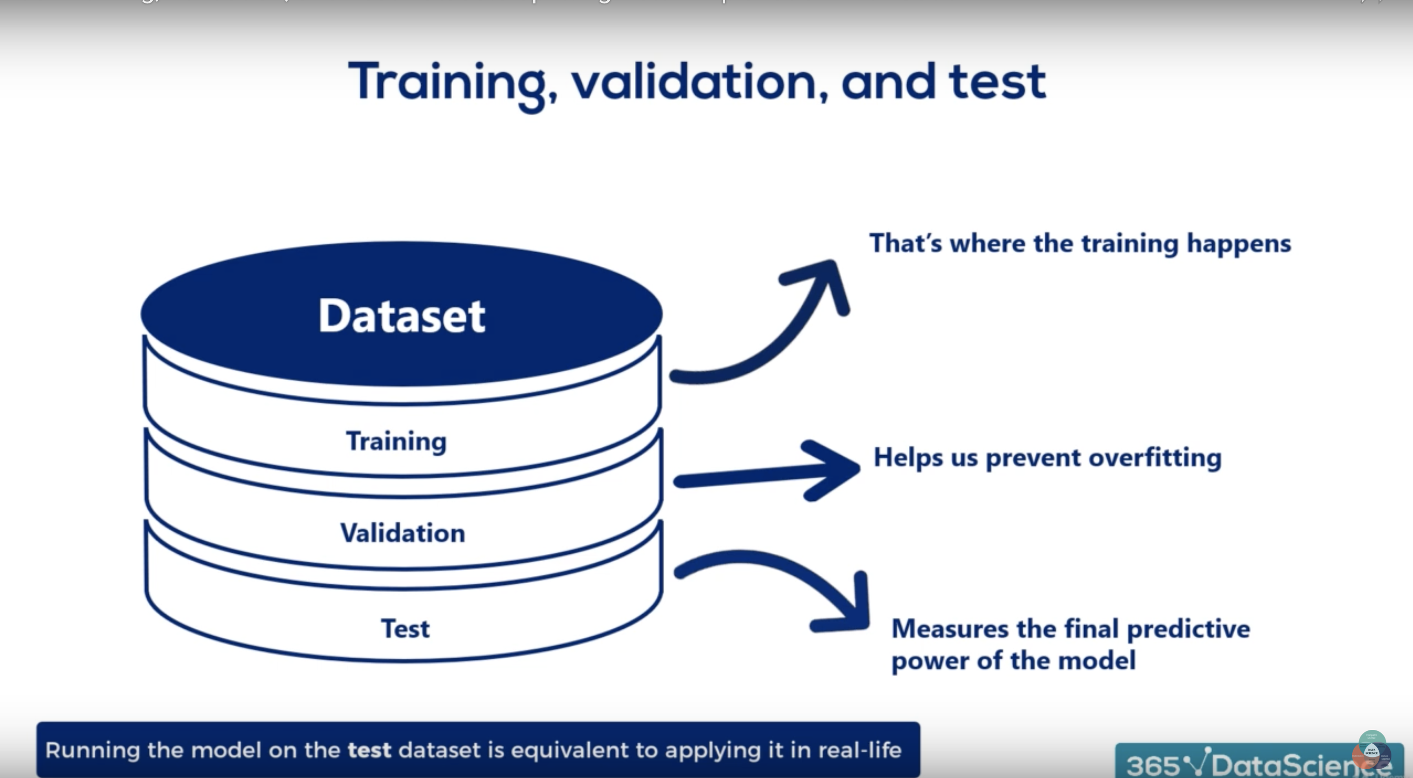
Splitting Data: Training, Testing, Validation**
- Training Set
- Labeled dataset
- Dataset used for training the model
- Validation Set
- Usually 80/10/10 split, where 10% is for validation set and 10% for test set
- Labeled dataset
- Dataset used for assessing the Model’s performance on each trained epoch
- The split between training and validation dataset is required to avoid model overfitting
- Overfitting happens when the Model is giving good results on the training data, however is not able to generalize on the data it has not been trained on.
- Giving good results on both training and validation dataset gives us greater confidence in the model and its ability to generalize
- Validation dataset should be representative
- Testing Set
- Measures the final predictive power of the Model
- Can be used to compare the performance of different models
Model Training: Bias Variance Tradeoff
Bias
- Indicates that the model is underfitting
- Caused by wrong assumptions, lack of complexity in the model
Variance
- Indicates that the model is overfitting
- Caused by over-complex models
- Model can be performing great on the testing set, but is not performing well on the validation set
$Total Error(x) = Bias^2 + Variance + Irreducible Error$
- As the model grows in complexity, it tends to move from Low Variance, High Bias to High Variance and Low Bias
- Best model is the model which keeps the Total Error minimal by making the right Bias-Variance tradeoff
- Examples of Improving the Model
- Adjusting the Model complexity
- Adjusting the training size
- Adjusting the Hyperparameters
Learning Curve
- Plots the model performance
- Training dataset and validation dataset error or accuracy against training set size
- scikit-learn provides
sklearn.learning_curve.learning_curve- Uses stratified k-fold cross validation by default
Model Debugging: Error Analysis
- Filter on failed predictions and manually look for patterns
- Pivot on target, key attributes, and failure type, and build histograms of error counts
- Common patterns
- Data problems (many variants for the same word)
- Labeling errors (data mislabeled)
- Under/over-represented subclasses (too many examples of one type)
- Discriminating information is not captured in features
- It often helps to look on what model is predicting correctly
Model Tuning: Regularization
- Regularization helps reduce variance / overfitting of the model
- Regularization penalizes for certain model complexity
- Higher complexity models are more likely to be unable to generalize well
- Regularization is achieved by adding a term to the loss function, that penalizes for the large weights: $loss + penalty$
- Regularization is another hyperparameter that should be found out based on k-fold cross validation
Regularization Techniques
Regularization in Linear Models
- L1 regularization, Lasso
$ penalty = \sum_{j=1}^{n} \lvert w_j \rvert $
- L2 regularization, Ridge
$ penalty = \sum_{j=1}^{n} \lvert w_j^2 \rvert $
L2 Regularization In Neural Network
$ penalty = (\sum_{j=1}^n \lvert w^{[j]} \rvert^2 ) \frac{\lambda}{2 m} $
$n$ - the number of layers $w^{[j]}$ - the weight matrix for the $j^th$ layer $m$ - the number of inputs $\lambda$ - the regularization parameter
Scikit Learn Support
- Ridge regression model: Linear regression with L2
sklearn.linear_model.Ridge
- Lasso regression model: Linear regression with L1
sklearn.linear_model.Lasso
- Elastic net regression model: Linear regression with both
sklearn.linear_model.ElasticNet
- Strength of regularization $c = \frac{1}{\alpha} $
Model Tuning: Hyperparameter Tuning
Parameter vs Hyperparameter
- Parameter: an internal configuration whose value can be estimated from the data
- Hyperparameter: an external configuration whose value cannot be estimated from the data
Tuning Hyperparameters
- Grid Search
- Will try all combinations for hyperparameters and evaluated the best
- Computationally intensive
- Random Search
- Finding the best set of hyperparameters based on random permutations of possible values of hyperparameters
Model Tuning
Training Data Tuning
Possible Issues and Solutions
- Small training data
- More data can be sampled and labeled if possible
- Training set biased against missing or more important scenarios
- Sample and label more data for those scenarios if possible
- Can’t easily sample or label more?
- Consider creating synthetic data (duplication or techniques like SMOTE)
- Training data doesn’t need to be exactly representative. Testing dataset needs to be exactly representative.
Feature Set Tuning
- Add features that help capture pattern for classes of errors
- Try different transformations of the same feature
- Apply dimensionality reduction to reduce impact of weak features
Dimensionality Reduction
- Common cause of overfitting: too many features for the amount of data
- Dimensaionality Reduction: Reduce the (effective) dimension of the data with minimal loss of information
- The curse of dimensionality: certain models may not be able to give good results in the current dimension due to sparsity of data
Model Tuning: Feature Extraction
- Mapping data into smaller feature space that captures the bulk of the information in the data
- aka Data compression
- Improves computational efficiency
- Reduces the curse of dimensionality
- Techniques
- Principal Component Analysis (PCA)
- Unsupervised Approach for feature extraction
- Linear Discriminant Analysis (LDA)
- Supervised Approach for feature extraction
- Kernel versions of these for fundamentally non-linear data
- Principal Component Analysis (PCA)
Feature Selection vs Feature Extraction
- Both Feature selection and Feature Extraction reduce the dimensionality of the feature space
- Feature Selection
- Uses algorithms to remove some of the features from the model
- Selected features will enable the model to have better performance
- There is no change (such as transform, linear combination or non-linear combination) in the selected features
- Feature Extraction
- Using algorithms to combine original features to generate a new set of features
- Number of features to be used in the model is generally less than the original number of features
Model Tuning: Bagging/Boosting
Bagging
- Good for high variance but low bias
- Generates group of weak learners that when combined together generate higher accuracy
- Create a x dataset of size m by randomly sampling original dataset with replacement (duplicates allowed)
- Train weak learners on the new datasets to generate predictions
- Choose the output by combining the individual predictions (average in regression problem) or voting (classification)
- Reduces variance
- Keeps bias the same
- sklearn
sklearn.ensemble.BaggingClassifiersklearn.ensemble.BaggingRegressor
Boosting
- Good for high bias and accepts weights on individual samples
- Assign strength to each week learner
- Iteratively train learners using misclassified examples by the previous weak learners
- Training a sequence of samples to get a strong model
- sklearn:
- sklearn.ensemble.AdaBoostClassifier
- sklearn.ensemble.AdaBoostRegressor
- sklearn.ensemble.GradientBoostingClassifier
- XGBoost library
Model Evaluation and Model Productionizing
Using ML Models in Production
- Integrating an ML solution with existing software
- Keeping it running successfully over time
Aspects to Consider
- Model hosting
- Model deployment
- Pipelines to provide feature vectors
- Code to provide low-latency and/or high-volume predictions
- Model and data update and versioning
- Quality monitoring and alarming
- Data and model security and encryption
- Customer privacy, fairness and trust
- Data provider contractual constraints
Types of Production Environments
- Batch Predictions
- All inputs are know upfront
- Predictions can be served real-time from pre-computed values
- Online Predictions
- Low latency requirements
- Online Training
- Data patterns change frequently, needs online training
Model Evaluation Metrics
Confusion Matrix
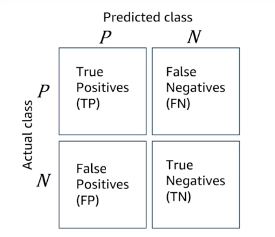
- Confusion Matrix values will be obtained when running the test data on the ML Model
Metrics
$ Accuracy = \frac{ TP + TN }{ TP + TN + FP + FN }$
$ Precision = \frac{ TP }{ TP + FP }$
$ Recall = \frac{ TP }{ TP + FN }$
$ F1-Score = \frac{ 2 x Precision x Recall }{ Precision + Recall }$
Cross Validation
Cross validation is a model validation technique, for assessing the prediction performance of the model. Based on this, certain chunk of data, referred to as testset, will be excluded from the training cycle and utilized for testing stage.
K-Fold Cross Validation
- K-fold gives you an opportunity to train across all the data
- Is especially useful for smaller data sets
- Typically 5-10 folds are used
Steps
- Randomly partition the data into k-segments
- For each segment / fold, train the model on all other segments exclusing the selectged one
- Use the fold excluded from training to evaluate the model
- Train on all the data
- Average metric across K-folds estimates test metric for trained model
Leave-one Out Cross Validation
- K = number of data points
- Used for very small sets
- K specifies the number of rows to used for training, and then leave one out
Stratified K-fold Cross Validation
- Preserve class proportions in the folds
- Used for imbalanced data
- There are seasonality or subgroups
Metrics for Linear Regression
$ Mean Squared Error $ $$ Mean Squared Error (MSE) = \frac{1}{N} \sum_{i=1}_{N} ( \hat{y_i} - y_i )^2 $$
$ R^2 $ $$ R^2 = 1 - \frac{Sum of Squared Error (SSE)}{Var(y)} $$
- $R^2$ Coefficient of Determination
- Values between 1 and 0
- 1 indcates that regression perfectly fits the data
$$ Adjusted R^2 = 1 - (1 - R^2) \frac{no. of data pts. - 1}{no. of data pts. - no. of variables - 1} $$
Using ML Models in Production: Storage
Considerations
- Read/Write speed, latency requirements
- Data Storage Format
- Platform-dependency
- Ability for schema to evolve
- Schema/data separability
- Type richness
- Scalability
Model and Pipeline Persistence
- Predictive Model Markup Language (PMML):
- Vendor-independent XML-based language for storing ML models
- Support varies in different libraries
- KNIME (analytics / ML Library): Full support
- Scikit-learn: extensive support
- Spark MLlib: Limited support
- Custom Methods:
- Scikit-learn: uses Python pickle method to serialize/deserialize Python objects
- Spark MLlib: transformers and estimators implement MLWritable
- TensorFlow: Allows saving of MetaGraph
- MxNet: Saves into JSON
Model Deployment
- A/B Testing
- May help detect production issues at early stage
- Shadow Testing
- Model is running behind the scenes
- Allows estimating Model’s performance while not serving production systems
Using ML Models in Production: Monitoring and Maintenance
Monitoring Considerations:
- Qualiy Metrics and Buinsess Impacts
- Dashboards
- Alarms
- User Feedback
- Continuous model performance reviews
Expected Changes
- The real-world domain may change over time
- The software environment may change
- High profile special cases may fail
- There may be a change in business goals
- Performance deterioration may require new tuning
- Changing goals may require new metrics
- Changing domain may require changes to validation set
- Your validation set may be replaced over time to avoid overfitting
Using ML Models in Production: Using AWS
- AWS SageMaker
- Pre-built notebooks
- Built-in, high performance algorithms
- One-click training
- Hyperparameter optimization
- One-click deployment
- Fully managed hosting with auto-scaling
- Amazon Rekognition Image
- Amazon Rekognition Video
- Amazon Lex
- Service for building conversational interfaces into any application using voice and text
- ASR (Automatic Speech Recognition)
- NLU (Natural Language Understanding)
-
Amazon Transcribe
- Amazon Polly
- Text to speech service
- Amazon Comprehend
- NLP (Natural Language Processing) service
- Discover insights and relationships in text
- Identify language based on the text
- Extract key phrases, places, people, brands or events
- Understand how positive or negative the text is
- Automatically organizes a collection of text files by topic
- NLP (Natural Language Processing) service
- Amazon Translate
- Automatic speech recognition (ASR) service
- AWS DeepLens
- Custom-designed deep learning inference engine
- HD video camera with on-board compute optimized for deep learning
- Integrates with AmazonSageMaker and AWS Lambda
- From inboxing to first inference in < 10 minutes
- Tutorials, examples, demos and pre-built models
- AWS Glue
- Data integration service for managing ETL jobs (Extract, Transform, Load)
- Deep Scalable Sparse Tensor Network Engine (DSSTNE): Neural network engine
Common Mistakes
- You solved the wrong problem
- The data was flawed
- The solution didn’t scale
- Final result doesn’t match with the prototype’s results
- It takes too long to fail
- The solution was too complicated
- There weren’t enough allocated engineering resources to try out long-term science ideas
- There was a lack of a true collaboration