Anomaly Detection: Isolation Forest Algorithm
Defining the Anomaly Detection Problem
- Data is set of vectors in d-dimensional space
- $x_1$, … $x_n$ each $x_i$ $\epsilon$ $R^d$
- Mixture of nominal points and anomaly points
- Anomaly points are generated by different generative process than the normal points
Solutions
- Supervised
- Training data labeled with “nominal” or “anomaly”
- Clean
- Training data are all “nominal”, test data contaminated with “anomaly” points
- Unsupervised
- Training data consists of mixture of “nominal” and “anomaly” points
Methods to Resolve Anomaly Detection Problem
- Density Based
- DBSCAN
- LOF
- Distance Based
- KNN
- K-MEANS
- Regression hyperplane distance
- Parametric
- GMM
- Single Class SVMs
- Extreme value theory
Well Defined Anomaly Distribution Assumption
-
WDAD: the anomalies are drawn from a well-defined probability distribution
-
The WDAD assumption is often risky
- adversarial situations (fraud, insider threats, cyber security)
- diverse set of potential causes
- user’s notion of anomaly changes with time
Isolation Forest Algorithm
- Builds an ensemble of random trees for a given data set
- Anomalies are points with the shortest average path length
- Assumes that outliers takes less steps to isolate compared to normal point in any data set
- Anomaly score is calculated for each point based on the formula: $2^{-E(h(x))/c(n)}$
- $h(x)$ is the number of edges in a tree for a point $x$
- $c(n)$ is a normalization constant for a data size of size $n$
- Isolation score can be used in both supervised and unsupervised setting
Algorithm Steps
- Sampling for Training
- Choose a sampling proportion from the original data set
- Generate a Binary Decision Tree
- Split based on 2 random elements
- Randomly choose an attribute
- Randomly choose a value of an attribute in its range of values
- Perform a split to branch the tree
- Split based on 2 random elements
- Repeat the process iteratively for the sub-data set
- After generating a Tree, repeat
- Create a Forest, collection of Trees
- Stop when maximum number of Trees is reached
- Feed data set an calculate anomaly score for each data point
- Calculate anomaly score for a data point across Tree, using the equation:
- $2^{-E(h(x))/c(n)}$
- Average out the calculated anomaly scores
- Calculate anomaly score for a data point across Tree, using the equation:
- Score Interpretation
- Anomalies will get a score closer to 1
- Scores much smaller than 0.5 indicates normal observations
- If all scores are close to 0.5 then the entire sample doesn’t seem to have clearly distinct anomalies
Example
In the following example we are using python’s sklearn library to experiment with the isolation forest algorithm. In the example below we are generating random data sets:
- Training Data Set
- Required to fit an estimator
- Test Data Set
- Testing Accuracy of the Isolation Forest Estimator
- Outlier Data Set
- Testing Accuracy in detecting outliers
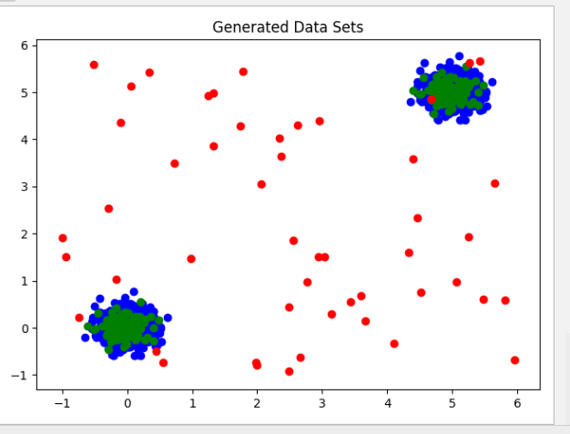
Generated Data:
# importing libaries ----
import numpy as np
import pandas as pd
import matplotlib.pyplot as plt
from pylab import savefig
from sklearn.ensemble import IsolationForest

# Instantiating container for Mersenne Twister pseudo-random number generator with a seed of int 42
rng = np.random.RandomState(42)

# Generating 2 clusters of data using "Standard Normal" distribution
# In Standard Normal distribution 95% of data lies within +-2
# Multiplying by 0.2 leaves 95% within +-0.4
X_train = 0.2 * rng.randn(1000, 2)
print((abs(X_train[:, 0]) <= 0.4).sum() / len(X_train[:, 0]) * 100,
      " percent of data lies within 2 devitations from the mean")
# Generating second cluster of data (5,5) points away from the center of the first cluster in both axes
X_train = np.r_[X_train + 5, X_train]

# Generating the Dest Data using the same distribution of the training data
X_test = 0.2 * rng.randn(100, 2)
# Second cluster of the Test Data as well
X_test = np.r_[X_test + 5, X_test]

# Generating outliers spread throughout the plot using uniform distribution
X_outlier = rng.uniform(low=-1, high=6, size=(50, 2))

# Visualizing the generated data sets: Training - blue, Test - green, Outliers - red
plt.title("Generated Data Sets")
plt.scatter(X_train[:, 0], X_train[:, 1], c='blue')
plt.scatter(X_test[:, 0], X_test[:, 1], c='green')
plt.scatter(X_outlier[:, 0], X_outlier[:, 1], c='red')
plt.show()

# Fitting the Isolation Forest Estimator with Training Data
# Contamination factors indicates the percentage of data we believe to be outliers
clf = IsolationForest(behaviour='new', max_samples=100, random_state=rng, contamination=0.1)
clf.fit(X_train)

# Running predictions on the Test and Outliers Data Sets using the estimator
pred_test = clf.predict(X_test)
pred_outlier = clf.predict(X_outlier)

print("Accuracy with Test Data: ", (pred_test == 1).sum() / len(pred_test))
print("Accuracy In Outlier Detection: ", (pred_outlier == -1).sum() / len(pred_outlier))